Tutorial 2: D to P Exciation in Helium
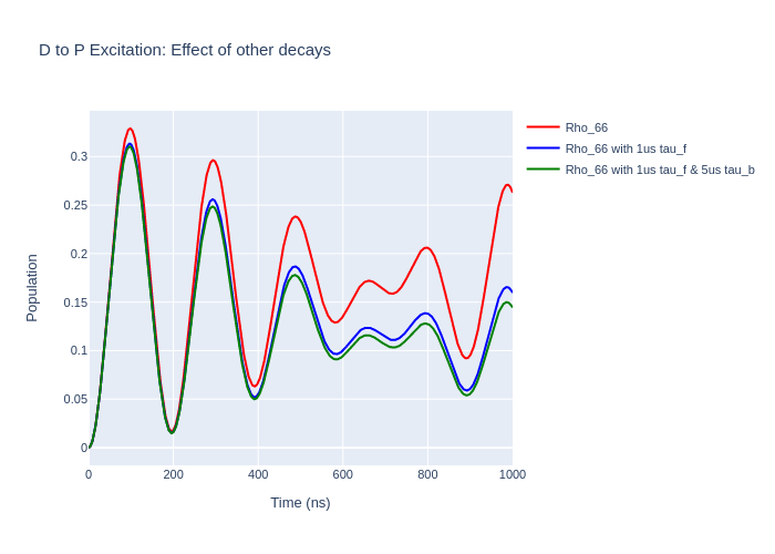
This tutorial demonstrates how to set up an excitation from a D state to a P state for Helium. The Helium D-state we are considering is now not the ground state of the atom so decay can occur to lower states. The upper P-state can also decay to other states non-radiatively which can also be modelled. In this tutorial the decay to other states is modelled.
The use of simultaneous polarisations and the normalisation of the half-Rabi frequencies is demonstrated here as well.
Also, the Wigner-D matrices are used to rotate the system to a different reference frame to show that this model is physically consistent in all reference frames.
Start by importing the libraries we will be using.
[1]:
import LASED as las
import numpy as np
from IPython.display import Image # This is to display html images in a notebook
import plotly.graph_objects as go
Decay to Other States
To set up a Laser-Atom system you must first declare the atomic states which you want to work with and label them. We are going to set up an example system for a D-state to a P-state transistion for helium where the P-state is a high principle quantum number Rydberg state. Therefore, we will assume that the wavelength of this fictitious transition is the ionisation energy of helium as this is a very high lying Rydberg state. This system is only for example purposes only and does not exist.

A level diagram of the system we will model is shown above.
The LaserAtomSystem is setup in the code block below. The decay (e.g. non-radiative decay) to other states outside the system from the excited state is characterised by the arrow from the upper states to state \(|f\rangle\). This can be modelled into the LaserAtomSystem using the keyword tau_f and inputting the lifetime of this decay. The decay to other states from the lower state is shown in the diagram by the arrow from the lower state to the state \(|b\rangle\). This can
be modelled using the keyword tau_b and inputting the lifetime of this decay.
We will excite this system with simultaneous right-hand circular and left-hand circular polarised light in the natural frame with the laser beam travelling down the quantisation axis. This will be linearly-polarised light in the collision frame where the transverse E-field of the laser is oscillating along the quantisation axis. Therefore, we must set Q = [-1, 1] and set the rabi_factors to [1, -1] as noted in Tutorial 1 and scale the Rabi frequency in the system by using
rabi_scaling. In this case set it to \(1/{\sqrt{2}}\).
Then, we create the sub-states and put them into either the ground or excited states.
[2]:
# System parameters
laser_wavelength = 900e-9 # wavelength of transition
w_e = las.angularFreq(laser_wavelength)

# Create states
one = las.State(label = 1, w = 0, m = -2, L = 2, S = 0)
two = las.State(label = 2, w = 0, m = -1, L = 2, S = 0)
three = las.State(label = 3, w = 0, m = 0, L = 2, S = 0)
four = las.State(label = 4, w = 0, m = 1, L = 2, S = 0)
five = las.State(label = 5, w = 0, m = 2, L = 2, S = 0)

six = las.State(label = 6, w = w_e, m = -1, L = 1, S = 0)
seven = las.State(label = 7, w = w_e, m = 0, L = 1, S = 0)
eight = las.State(label = 8, w = w_e, m = 1, L = 1, S = 0)

G = [one, two, three, four, five] # ground states
E = [six, seven, eight] # excited states
Q = [-1, 1] # laser radiation polarisation
rabi_scaling_he = 1/np.sqrt(2)
rabi_factors_he = [1, -1]
laser_intensity = 100 # mW/mm^2
tau = 60e3 # lifetime in ns (estimated)
tau_f = 1000 # non-radiative lifetime of rydberg upper state to other high-lying states (ns)
tau_b = 5000  # non-radiatuve lifetime of metastable D-state (ns)
Set the simulation time for 1000 ns every 1 ns as follows:
[3]:
# Simulation parameters
start_time = 0
stop_time = 1000 # in ns
time_steps = 1001
time = np.linspace(start_time, stop_time, time_steps)
Create the LaserAtomSystem object. To set the initial conditions of the density matrix at t = 0 ns \(\rho(t = 0)\) we can use the setRho_0(s1, s2, val) where s1 and s2 are State objects denoting the element of the density matrix to be set as \(\rho_{s1,s2}\) and val denotes the value assigned to this element.
For this system we have set the populations of states \(|1\rangle\), \(|3\rangle\), and \(|5\rangle\) as 1/3. So the density matrix elements \(\rho_{11}\) = \(\rho_{33}\) = \(\rho_{55}\) = 1/3.
[4]:
helium_system = las.LaserAtomSystem(E, G, tau, Q, laser_wavelength,
                                    laser_intensity = laser_intensity, rabi_scaling = rabi_scaling_he,
                                    rabi_factors = rabi_factors_he)
helium_system_tauf = las.LaserAtomSystem(E, G, tau, Q, laser_wavelength,
                                         tau_f = tau_f,
                                    laser_intensity = laser_intensity, rabi_scaling = rabi_scaling_he,
                                    rabi_factors = rabi_factors_he)
helium_system_tauf_taub = las.LaserAtomSystem(E, G, tau, Q, laser_wavelength,
                                         tau_f = tau_f, tau_b = tau_b,
                                    laser_intensity = laser_intensity, rabi_scaling = rabi_scaling_he,
                                    rabi_factors = rabi_factors_he)
helium_system.setRho_0(one, one, 1/3)
helium_system.setRho_0(three, three, 1/3)
helium_system.setRho_0(five, five, 1/3)
helium_system_tauf.setRho_0(one, one, 1/3)
helium_system_tauf.setRho_0(three, three, 1/3)
helium_system_tauf.setRho_0(five, five, 1/3)
helium_system_tauf_taub.setRho_0(one, one, 1/3)
helium_system_tauf_taub.setRho_0(three, three, 1/3)
helium_system_tauf_taub.setRho_0(five, five, 1/3)
Time evolve the system.
[5]:
helium_system.timeEvolution(time)
helium_system_tauf.timeEvolution(time)
helium_system_tauf_taub.timeEvolution(time)
Now, we can plot the populations using Plotly (or any other plotting package).
[6]:
rho_66 = [ abs(rho) for rho in helium_system.Rho_t(six, six)]
rho_66_tauf = [abs(rho) for rho in helium_system_tauf.Rho_t(six, six)]
rho_66_tauf_taub = [abs(rho) for rho in helium_system_tauf_taub.Rho_t(six, six)]

fig_upper = go.Figure(data = go.Scatter(x = time,
                                 y = rho_66,
                                 mode = 'lines',
                                    name = "Rho_66",
                                    marker = dict(
                                color = 'red',
                                symbol = 'x',
                            )))

fig_upper.add_trace(go.Scatter(x = time,
                                 y = rho_66_tauf,
                                 mode = 'lines',
                                    name = "Rho_66 with 1us tau_f",
                                    marker = dict(
                                color = 'blue',
                                symbol = 'square',
                           )))
fig_upper.add_trace(go.Scatter(x = time,
                                 y = rho_66_tauf_taub,
                                 mode = 'lines',
                                    name = "Rho_66 with 1us tau_f & 5us tau_b",
                                    marker = dict(
                                color = 'green',
                                symbol = 'circle',
                           )))

fig_upper.update_layout(showlegend = True,
                       title = "D to P Excitation: Effect of other decays",
                     xaxis_title = "Time (ns)",
                     yaxis_title = "Population",
                    font = dict(
                        size = 11))
fig_upper.write_image("SavedPlots/tutorial2-HeLifetimes.png")
fig_upper.write_image("SavedPlots/tutorial2-HeLifetimes.svg")
Image("SavedPlots/tutorial2-HeLifetimes.png")
[6]:
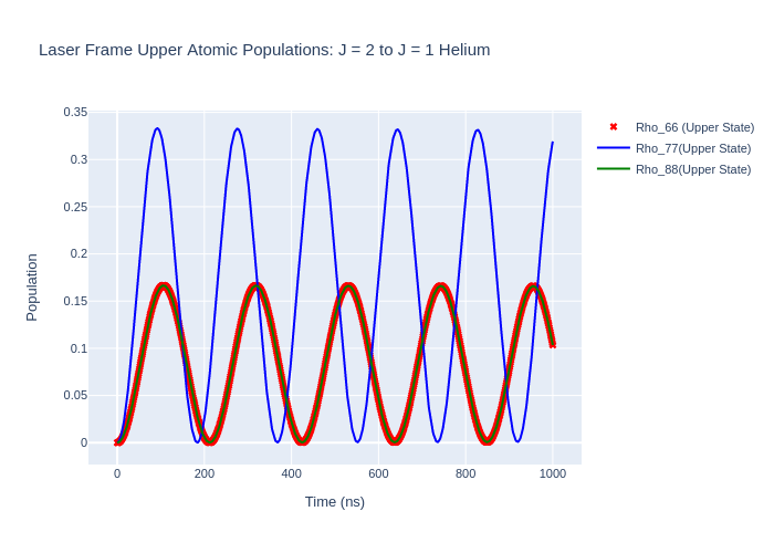
Rotation
With LASED we can rotate density matrices to different reference frames using the Wigner-D matrix.
Note: The Wigner-D matrix is only defined for J-represenattion (when isospin I = 0) and therefore when in F-representation the rotation may not be correct. Also, density matrices can only be rotated for single atomic states so the optical coherences between ground and excited states cannot be rotated. To obtain optical coherences in a different reference frame the initial density matrix (at t = 0) must be rotated and time evolved with the polarisation rotated to that frame.
The rotation is defined by Euler angles alpha, beta, and gamma. The frame is rotated with each angle in succession so that: - alpha is the rotation (in radians) around the initial z-axis to obtain the new frame Z’ - beta is the rotation (in radians) about the new y’-axis to obtain the new frame Z’’ - gamma is the rotation (in radians) about the new z’’-axis to obtain the final frame
In LASED to rotate the initial density matrix use rotateRho_0(alpha, beta, gamma) on the LaserAtomSystem. In this he lium system the atom is changed to be defined in the collision frame from the natural frame so the polarisation is changed to be purely linear with Q = [0] and scaled to 1.
Note: To simulate a linear polarisation with an angle with respect to the x-axis we can initialise the density matrix in that frame, rotate to the collision frame (with the polarisation aligned with the x-axis, time evolve the system, and then rotate back to the frame where the polarisation is at an angle.
[7]:
alpha = np.pi/2  # Angles are in radians
beta = np.pi/2
gamma = -np.pi/2
helium_system_rot = helium_system
helium_system_rot.rotateRho_0(alpha, beta, gamma)
helium_system_rot.Q = [0]
helium_system_rot.rabi_scaling = 1
helium_system_rot.rabi_factors = [1]
Now, we can time evolve this system in this new reference frame.
[8]:
print(helium_system_rot)
helium_system_rot.timeEvolution(time)
LaserAtomSystem([6, 7, 8], [1, 2, 3, 4, 5], 60000.0, [0], [1, 0, -1], 9e-07, None, 100, None)
Now we can plot what the populations look like.
[9]:
las_sys = helium_system_rot
rho_66 = [ abs(rho) for rho in las_sys.Rho_t(six, six)]
rho_77 = [abs(rho) for rho in las_sys.Rho_t(seven, seven)]
rho_88 = [abs(rho) for rho in las_sys.Rho_t(eight, eight)]

fig_upper = go.Figure(data = go.Scatter(x = time,
                                 y = rho_66,
                                 mode = 'markers',
                                    name = "Rho_66 (Upper State)",
                                    marker = dict(
                                color = 'red',
                                symbol = 'x',
                            )))

fig_upper.add_trace(go.Scatter(x = time,
                                 y = rho_77,
                                 mode = 'lines',
                                    name = "Rho_77(Upper State)",
                                    marker = dict(
                                color = 'blue',
                                symbol = 'square',
                           )))
fig_upper.add_trace(go.Scatter(x = time,
                                 y = rho_88,
                                 mode = 'lines',
                                    name = "Rho_88(Upper State)",
                                    marker = dict(
                                color = 'green',
                                symbol = 'circle',
                           )))

fig_upper.update_layout(title = "Laser Frame Upper Atomic Populations: J = 2 to J = 1 Helium",
                 xaxis_title = "Time (ns)",
                 yaxis_title = "Population",
                font = dict(
                    size = 11))

fig_upper.write_image("SavedPlots/tutorial2-HeFigUpperCollFrame.png")
Image("SavedPlots/tutorial2-HeFigUpperCollFrame.png")
[9]:
[10]:
rho11 = [ abs(rho) for rho in las_sys.Rho_t(one, one)]
rho22 = [ abs(rho) for rho in las_sys.Rho_t(two, two)]
rho33 = [ abs(rho) for rho in las_sys.Rho_t(three, three)]
rho44 = [ abs(rho) for rho in las_sys.Rho_t(four, four)]
rho55 = [ abs(rho) for rho in las_sys.Rho_t(five, five)]
fig_lower = go.Figure(data = go.Scatter(x = time,
y = rho11,
mode = 'lines',
name = "Rho_11 (Lower State)",
marker = dict(
color = 'red',
symbol = 'circle',
)))
fig_lower.add_trace(go.Scatter(x = time,
y = rho22,
mode = 'markers',
name = "Rho_22 (Lower State)",
marker = dict(
color = 'blue',
symbol = 'x',
)))
fig_lower.add_trace(go.Scatter(x = time,
y = rho33,
mode = 'lines',
name = "Rho_33 (Lower State)",
marker = dict(
color = 'purple',
symbol = 'x',
)))
fig_lower.add_trace(go.Scatter(x = time,
y = rho44,
mode = 'lines',
name = "Rho_44 (Lower State)",
marker = dict(
color = 'gold',
symbol = 'x',
)))
fig_lower.add_trace(go.Scatter(x = time,
y = rho55,
mode = 'lines',
name = "Rho_55 (Lower State)",
marker = dict(
color = 'green',
symbol = 'square',
)))
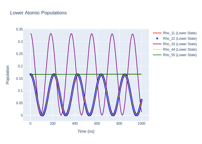
fig_lower.update_layout(title = "Lower Atomic Populations",
xaxis_title = "Time (ns)",
yaxis_title = "Population")
fig_lower.write_image("SavedPlots/tutorial2-HeFigLowerCollFrame.png")
Image("SavedPlots/tutorial2-HeFigLowerCollFrame.png")
[10]:
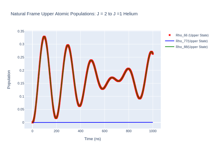
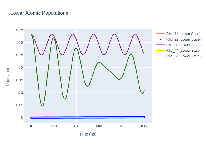
If we rotate the time-evolved density matrix rho_t back to the natural frame we should get the same populations as when we evolved in the natural frame as the excitation must be the same in all reference frames. We can do this rotation by using rotateRho_t on the LaserAtomSystem.
Note: A message will be thrown saying that the optical coherences are not rotated.
[11]:
helium_system_rot.rotateRho_t(alpha, -beta, gamma)
Now we can plot the results and obtain the same plots as in the first time evolution.
[12]:
las_sys = helium_system_rot
rho_66 = [ abs(rho) for rho in las_sys.Rho_t(six, six)]
rho_77 = [abs(rho) for rho in las_sys.Rho_t(seven, seven)]
rho_88 = [abs(rho) for rho in las_sys.Rho_t(eight, eight)]

fig_upper = go.Figure(data = go.Scatter(x = time,
                                 y = rho_66,
                                 mode = 'markers',
                                    name = "Rho_66 (Upper State)",
                                    marker = dict(
                                color = 'red',
                                symbol = 'x',
                            )))

fig_upper.add_trace(go.Scatter(x = time,
                                 y = rho_77,
                                 mode = 'lines',
                                    name = "Rho_77(Upper State)",
                                    marker = dict(
                                color = 'blue',
                                symbol = 'square',
                           )))
fig_upper.add_trace(go.Scatter(x = time,
                                 y = rho_88,
                                 mode = 'lines',
                                    name = "Rho_88(Upper State)",
                                    marker = dict(
                                color = 'green',
                                symbol = 'circle',
                           )))

fig_upper.update_layout(title = "Natural Frame Upper Atomic Populations: J = 2 to J =1 Helium",
                 xaxis_title = "Time (ns)",
                 yaxis_title = "Population",
                font = dict(
                    size = 11))

fig_upper.write_image("SavedPlots/tutorial2-HeFigUpperRotatedToNatFrame.png")
Image("SavedPlots/tutorial2-HeFigUpperRotatedToNatFrame.png")
[12]:
[13]:
rho11 = [ abs(rho) for rho in las_sys.Rho_t(one, one)]
rho22 = [ abs(rho) for rho in las_sys.Rho_t(two, two)]
rho33 = [ abs(rho) for rho in las_sys.Rho_t(three, three)]
rho44 = [ abs(rho) for rho in las_sys.Rho_t(four, four)]
rho55 = [ abs(rho) for rho in las_sys.Rho_t(five, five)]


fig_lower = go.Figure(data = go.Scatter(x = time,
                                 y = rho11,
                                 mode = 'lines',
                                    name = "Rho_11 (Lower State)",
                                    marker = dict(
                                color = 'red',
                                symbol = 'circle',
                            )))
fig_lower.add_trace(go.Scatter(x = time,
                                 y = rho22,
                                 mode = 'markers',
                                    name = "Rho_22 (Lower State)",
                                    marker = dict(
                                color = 'blue',
                                symbol = 'x',
                            )))
fig_lower.add_trace(go.Scatter(x = time,
                                 y = rho33,
                                 mode = 'lines',
                                    name = "Rho_33 (Lower State)",
                                    marker = dict(
                                color = 'purple',
                                symbol = 'x',
                            )))
fig_lower.add_trace(go.Scatter(x = time,
                                 y = rho44,
                                 mode = 'lines',
                                    name = "Rho_44 (Lower State)",
                                    marker = dict(
                                color = 'gold',
                                symbol = 'x',
                            )))
fig_lower.add_trace(go.Scatter(x = time,
                                 y = rho55,
                                 mode = 'lines',
                                    name = "Rho_55 (Lower State)",
                                    marker = dict(
                                color = 'green',
                                symbol = 'square',
                            )))
fig_lower.update_layout(title = "Lower Atomic Populations",
                        xaxis_title = "Time (ns)",
                 yaxis_title = "Population")

fig_lower.write_image("SavedPlots/tutorial2-HeFigLowerRotatedToNatFrame.png")
Image("SavedPlots/tutorial2-HeFigLowerRotatedToNatFrame.png")
[13]:
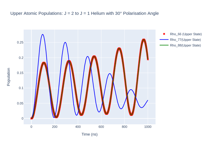
Polarisation Angle
The polarisation angle in LASED is assumed to be 0 during excitation i.e. the polarisation vector is in the same direction as the quantisation axis (QA). To model a non-zero polarisation angle with respect to the QA the LaserAtomSystem() must be rotated by the polarisation angle \(\theta\) to the frame where the polarisation is in the direction of the QA, time evolved using timeEvolution() and then rotated back to the old frame (so rotate by -\(\theta\)).
As an example, the Helium system will be excited by liner light polarised at an angle of \(30^{\circ}\) to the QA. To do this rotate the He system by \((\alpha, \beta, \gamma)\) = (90:math:^{circ}, 30\(^{\circ}\), -90:math:^{circ}), excite with polarisation Q = [0], and then rotate the system back to the old reference frame by performing the rotation (90:math:^{circ}, -30:math:^{circ}, -90:math:^{circ}).
Rotate the Helium system and time evolve using a linear polarisation:
[14]:
theta = 30 # Polarisation angle
alpha = np.pi/2
beta = 30*np.pi/180  # Convert to radians
gamma = -np.pi/2

# Set up the laser-atom system
helium_system_polarisation_angle = helium_system_rot
helium_system_polarisation_angle.rotateRho_0(alpha, beta, gamma)

# Time evolve and plot
helium_system_polarisation_angle.timeEvolution(time)

# Rotate rho_t back to the original reference frame (the optical coherences will not be preserved)
helium_system_polarisation_angle.rotateRho_t(alpha, -beta, gamma)
[15]:
las_sys = helium_system_polarisation_angle
rho_66 = [ abs(rho) for rho in las_sys.Rho_t(six, six)]
rho_77 = [abs(rho) for rho in las_sys.Rho_t(seven, seven)]
rho_88 = [abs(rho) for rho in las_sys.Rho_t(eight, eight)]

fig_upper = go.Figure(data = go.Scatter(x = time,
                                 y = rho_66,
                                 mode = 'markers',
                                    name = "Rho_66 (Upper State)",
                                    marker = dict(
                                color = 'red',
                                symbol = 'x',
                            )))

fig_upper.add_trace(go.Scatter(x = time,
                                 y = rho_77,
                                 mode = 'lines',
                                    name = "Rho_77(Upper State)",
                                    marker = dict(
                                color = 'blue',
                                symbol = 'square',
                           )))
fig_upper.add_trace(go.Scatter(x = time,
                                 y = rho_88,
                                 mode = 'lines',
                                    name = "Rho_88(Upper State)",
                                    marker = dict(
                                color = 'green',
                                symbol = 'circle',
                           )))

fig_upper.update_layout(title = f"Upper Atomic Populations: J = 2 to J = 1 Helium with {theta}° Polarisation Angle",
                 xaxis_title = "Time (ns)",
                 yaxis_title = "Population",
                font = dict(
                    size = 11))
fig_upper.write_image("SavedPlots/tutorial2-HePolarisationAngle.png")
Image("SavedPlots/tutorial2-HePolarisationAngle.png")
[15]: