Tutorial 3: He Excitation: Initialisation with Data and Angular Shape
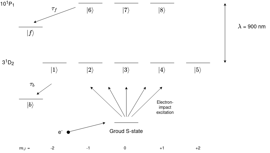
In this tutorial a more relaistic system will be simulated which could be the process in an experiment and the angular shape of the electron cloud will be plotted and a video of the angular shape of the electron cloud over time will be plotted. Let’s say that helium is excited to the 3D-state via electron impact from its ground state whilst a laser excites these electron-excited atoms into a high-lying 10P-state. A level diagram of the system is shown below.
Let’s import all the libraries needed. We will need a library to read in data from a datafile. pandas is a good library to do this.
[1]:
import LASED as las
import numpy as np
import plotly.graph_objects as go
from IPython.display import Image # This is to display html images in a notebook
import pandas as pd  #This librray is used to read in the data
Setting up the System
This is a very similar system to last tutorial except for the lifetime and laser wavelength. Both of these values are taken from looking at the transition on the National Institute of Standards and Technology’s (NIST) atomic database. The page for He can be found here. The 10P state data is found here and the 3D data is found here.
To calculate the total lifetime for \(\tau_f\) and \(\tau_b\) sum the decay rates \(A_{ki}\) for each transition from the upper state and lower state to states not in the laser-excitation and then take the reciprocal of this to get the total lifetime. For example, \(\tau_f\) for the 10P state of He has many decays to lower states however the largest decay rates will contribute the most so the first three are
[2]:
tau = 80.7e3 # lifetime in ns (take from NIST 1/A_ki as this is in rad/s)
tau_f = 59.6 # lifetime of upper state to other states in ns
tau_b = 15.7 # lifetime of lower state decay to other states in ns
laser_wavelength = 900e-9 # wavelength of laser 3D to 9P state from NIST

w_e = las.angularFreq(laser_wavelength)  # Converted to angular frequency in Grad/s

# Create states for J = 2 -> J = 1
one = las.State(L = 2, S = 0, m = -2, w = 0, label = 1)
two = las.State(L = 2, S = 0, m = -1, w = 0, label = 2)
three = las.State(L = 2, S = 0, m = 0, w = 0, label = 3)
four = las.State(L = 2, S = 0, m = 1, w = 0, label = 4)
five = las.State(L = 2, S = 0, m = 2, w = 0, label = 5)
six = las.State(L = 1, S = 0, m = -1, w = w_e, label = 6)
seven = las.State(L = 1, S = 0, m = 0, w = w_e, label = 7)
eight = las.State(L = 1, S = 0, m = 1, w = w_e, label = 8)

G = [one, two, three, four, five] # ground states
E = [six, seven, eight] # excited states
Q = [0] # laser radiation polarisation

# Simulation parameters
start_time = 0
stop_time = 200 # in ns
steps = 201
time = np.linspace(start_time, stop_time, steps)

# Laser parameters
laser_intensity = 1500 # laser intensity in mW/mm^2
Next, make the LaserAtomSystem.
[3]:
helium_system = las.LaserAtomSystem(E, G, tau, Q, laser_wavelength, tau_f = tau_f,
                                 tau_b = tau_b, laser_intensity = laser_intensity)
Initialisating the Laser-Atom System with Data
Now, we need to extract the data from the datafile. This is scattering amplitude data kindly given by Igor Brey who has calculated these amplitudes from a model. The model is quite accurate for helium and gives amplitudes for various impact angles.
Igor calculated electron impact excitation amplitudes for all angles to the 3\(^1\)D\(_2\) state. With this data we can generate an initial density matrix to excite from real data. The data was generated in the collison frame.
The density matrix elements correspond to \(\rho_{M,M'} = \sum_{m'}{\langle}Mm'_f|\rho_f|M'm'_f{\rangle} = {\langle}f(M)f^*(M'){\rangle}\)
where \(f(M)\) is the scattering amplitude for state \(|J M \rangle\).
Select data from the scattering angle of 45 degrees.
[4]:
scat_data = pd.read_csv("31DAmplitudes.csv")
scat_angle_data = scat_data.loc[scat_data['Angle'] == 45]
print(scat_angle_data)
    Angle  Re a(+2)*1e-12  Im(a+2)*1e-12  Re a(+1)*1e-12  Im(a+1)*1e-12  \
45     45           8.821           19.5           14.84         -35.66

    Re a(0)*1e-12  Im(a0)*1e-12  Re(a-1)*1e-12  Im(a-1)*1e-12  Re(a-2)*1e-12  \
45          85.82        -12.27         -14.84          35.66          8.821

    Im(a-2)*1e-12
45           19.5
Now we have read in what values the amplitudes are and we can now obtain the diagonal density matrix elements. First, put the scattering amplitudes in variables and put them into a list.
[5]:
f_2 = scat_angle_data.iloc[0].at["Re a(+2)*1e-12"] + scat_angle_data.iloc[0].at["Im(a+2)*1e-12"]*1.j
f_1 = scat_angle_data.iloc[0].at["Re a(+1)*1e-12"] + scat_angle_data.iloc[0].at["Im(a+1)*1e-12"]*1.j
f_0 = scat_angle_data.iloc[0].at["Re a(0)*1e-12"] + scat_angle_data.iloc[0].at["Im(a0)*1e-12"]*1.j
f_minus1 = scat_angle_data.iloc[0].at["Re(a-1)*1e-12"] + scat_angle_data.iloc[0].at["Im(a-1)*1e-12"]*1.j
f_minus2 = scat_angle_data.iloc[0].at["Re(a-2)*1e-12"] + scat_angle_data.iloc[0].at["Im(a-2)*1e-12"]*1.j
f = [f_minus2, f_minus1, f_0, f_1, f_2]
Now, calculate the density matrix \(\rho\). Normalise the populations so that tr(𝜌) = 1.
Note: The density matrix created must be in the order with the value of \(\rho_{-m, -m}\) starting the upper left-hand side of the matrix to \(\rho_{m, m}\) at the bottom right-hand corner. \(m\) is the projection of the total angular momentum.
[6]:
rho_collision = np.zeros((len(G), len(G)), dtype = complex)

for i, population in enumerate(f):
    for j, population in enumerate(f):
        rho_collision[i][j] = f[i]*np.conj(f[j])

# Normalisation
norm = 0
for i in range(len(G)):
    norm += rho_collision[i][i]
rho_collision = rho_collision/norm
print("The J = 2 density matrix in the collision frame is \n", pd.DataFrame(np.flip(rho_collision)))
The J = 2 density matrix in the collision frame is
                     0                   1                   2  \
0  0.040126+0.000000j -0.049448+0.052905j  0.045355+0.156080j
1 -0.049448-0.052905j  0.130688+0.000000j  0.149895-0.252136j
2  0.045355-0.156080j  0.149895+0.252136j  0.658372+0.000000j
3  0.049448+0.052905j -0.130688+0.000000j -0.149895+0.252136j
4  0.040126+0.000000j -0.049448+0.052905j  0.045355+0.156080j

                    3                   4
0  0.049448-0.052905j  0.040126+0.000000j
1 -0.130688+0.000000j -0.049448-0.052905j
2 -0.149895-0.252136j  0.045355-0.156080j
3  0.130688+0.000000j  0.049448+0.052905j
4  0.049448-0.052905j  0.040126+0.000000j
Note: Above pandas is used to convert the matrix into a DataFrame just for display purposes and the display of a matrix as a DataFrame is neater and the indeces are easier to read.
Now, we must initialise the density matrix of the LaserAtomSystem with this calculated ground state density matrix. To do this, we can use the function appendDensityMatrixToRho_0(density_rho, state_type) where: * rho_0 is a column vector which is of size n\(^2\), where n is the number of energy levels in the system. This column vector represents the denisty matrix for the laser-atom system. It is flattened (one-dimensional) as it is easier to solve the equations of motion
generated with this form. It is in the form of:
density_rhois the density matrix of the ground or upper state density matrix to be input into the flattened coupled denisty matrix and then initialised asrho_0in theLaserAtomSystem. This is of typendarray. This is a usual 2D matrix.state_typeis a character of ‘e’ or ‘g’ for appending the excited state density matrix or ‘g’ for the ground state density matrix.
rho_0 is already initialised as empty with the correct size when a LaserAtomSystem is initialised.
[7]:
helium_system.appendDensityMatrixToRho_0(rho_collision, "g")
print("The initial ρ for the laser-atom system is: \n", helium_system.rho_0)
The initial ρ for the laser-atom system is:
 [[ 0.04012626+0.j        ]
 [ 0.0494475 -0.05290513j]
 [ 0.04535541+0.15607978j]
 [-0.0494475 +0.05290513j]
 [ 0.04012626+0.j        ]
 [ 0.        +0.j        ]
 [ 0.        +0.j        ]
 [ 0.        +0.j        ]
 [ 0.0494475 +0.05290513j]
 [ 0.1306877 +0.j        ]
 [-0.1498946 +0.25213635j]
 [-0.1306877 +0.j        ]
 [ 0.0494475 +0.05290513j]
 [ 0.        +0.j        ]
 [ 0.        +0.j        ]
 [ 0.        +0.j        ]
 [ 0.04535541-0.15607978j]
 [-0.1498946 -0.25213635j]
 [ 0.65837208+0.j        ]
 [ 0.1498946 +0.25213635j]
 [ 0.04535541-0.15607978j]
 [ 0.        +0.j        ]
 [ 0.        +0.j        ]
 [ 0.        +0.j        ]
 [-0.0494475 -0.05290513j]
 [-0.1306877 +0.j        ]
 [ 0.1498946 -0.25213635j]
 [ 0.1306877 +0.j        ]
 [-0.0494475 -0.05290513j]
 [ 0.        +0.j        ]
 [ 0.        +0.j        ]
 [ 0.        +0.j        ]
 [ 0.04012626+0.j        ]
 [ 0.0494475 -0.05290513j]
 [ 0.04535541+0.15607978j]
 [-0.0494475 +0.05290513j]
 [ 0.04012626+0.j        ]
 [ 0.        +0.j        ]
 [ 0.        +0.j        ]
 [ 0.        +0.j        ]
 [ 0.        +0.j        ]
 [ 0.        +0.j        ]
 [ 0.        +0.j        ]
 [ 0.        +0.j        ]
 [ 0.        +0.j        ]
 [ 0.        +0.j        ]
 [ 0.        +0.j        ]
 [ 0.        +0.j        ]
 [ 0.        +0.j        ]
 [ 0.        +0.j        ]
 [ 0.        +0.j        ]
 [ 0.        +0.j        ]
 [ 0.        +0.j        ]
 [ 0.        +0.j        ]
 [ 0.        +0.j        ]
 [ 0.        +0.j        ]
 [ 0.        +0.j        ]
 [ 0.        +0.j        ]
 [ 0.        +0.j        ]
 [ 0.        +0.j        ]
 [ 0.        +0.j        ]
 [ 0.        +0.j        ]
 [ 0.        +0.j        ]
 [ 0.        +0.j        ]]
Time Evolution
Model the polarisation at 30\(^{\circ}\) to the QA so rotate the system, then time evolve, and then rotate back.
[8]:
# Rotate by (90°, 30°, -90°)
theta = 30
alpha = np.pi/2
beta = theta*np.pi/180
gamma = -np.pi/2
helium_system.rotateRho_0(alpha, beta, gamma)
Time evolve:
[9]:
helium_system.timeEvolution(time)
Rotate back:
[10]:
# Rotate by (90°, -30°, -90°)
helium_system.rotateRho_t(alpha, -beta, gamma)
Plotting and Saving Data
Now, save and plot the data.
[11]:
helium_system.saveToCSV("SavedData/MetastableHeBrey1500mW.csv")
[12]:
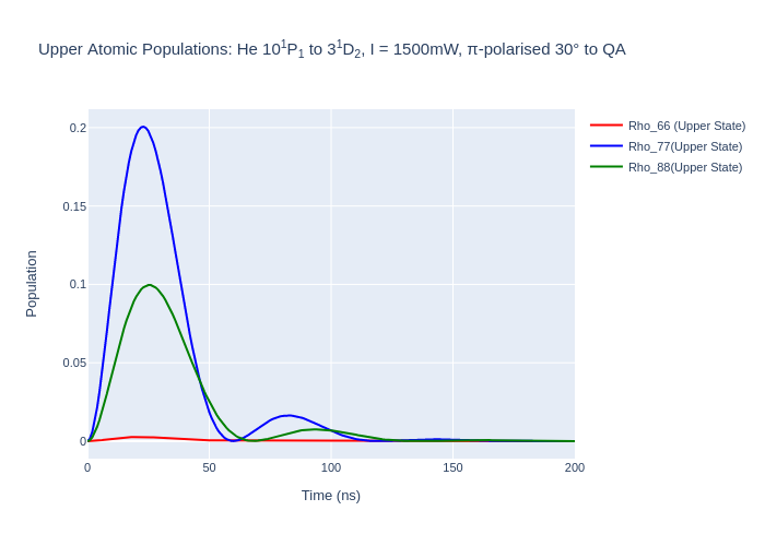
rho_66 = [ abs(rho) for rho in helium_system.Rho_t(six, six)]
rho_77 = [abs(rho) for rho in helium_system.Rho_t(seven, seven)]
rho_88 = [abs(rho) for rho in helium_system.Rho_t(eight, eight)]

fig_upper = go.Figure(data = go.Scatter(x = time,
                                 y = rho_66,
                                 mode = 'lines',
                                    name = "Rho_66 (Upper State)",
                                    marker = dict(
                                color = 'red',
                                symbol = 'x',
                            )))

fig_upper.add_trace(go.Scatter(x = time,
                                 y = rho_77,
                                 mode = 'lines',
                                    name = "Rho_77(Upper State)",
                                    marker = dict(
                                color = 'blue',
                                symbol = 'square',
                           )))
fig_upper.add_trace(go.Scatter(x = time,
                                 y = rho_88,
                                 mode = 'lines',
                                    name = "Rho_88(Upper State)",
                                    marker = dict(
                                color = 'green',
                                symbol = 'circle',
                           )))

fig_upper.update_layout(title = "Upper Atomic Populations: He 10<sup>1</sup>P<sub>1</sub> to 3<sup>1</sup>D<sub>2</sub>, I = {:0.0f}mW, π-polarised 30° to QA".format(laser_intensity, tau/1e3, tau_f/1e3),
                 xaxis_title = "Time (ns)",
                 yaxis_title = "Population",
                font = dict(
                    size = 11))

fig_upper.write_image("SavedPlots/tutorial3-HeFigUpper.png")
Image("SavedPlots/tutorial3-HeFigUpper.png")
[12]:
[13]:
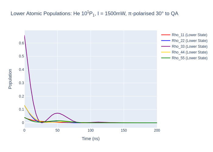
rho11 = [ abs(rho) for rho in helium_system.Rho_t(one, one)]
rho22 = [ abs(rho) for rho in helium_system.Rho_t(two, two)]
rho33 = [ abs(rho) for rho in helium_system.Rho_t(three, three)]
rho44 = [ abs(rho) for rho in helium_system.Rho_t(four, four)]
rho55 = [ abs(rho) for rho in helium_system.Rho_t(five, five)]


fig_lower = go.Figure(data = go.Scatter(x = time,
                                 y = rho11,
                                 mode = 'lines',
                                    name = "Rho_11 (Lower State)",
                                    marker = dict(
                                color = 'red',
                                symbol = 'circle',
                            )))
fig_lower.add_trace(go.Scatter(x = time,
                                 y = rho22,
                                 mode = 'lines',
                                    name = "Rho_22 (Lower State)",
                                    marker = dict(
                                color = 'blue',
                                symbol = 'x',
                            )))
fig_lower.add_trace(go.Scatter(x = time,
                                 y = rho33,
                                 mode = 'lines',
                                    name = "Rho_33 (Lower State)",
                                    marker = dict(
                                color = 'purple',
                                symbol = 'x',
                            )))
fig_lower.add_trace(go.Scatter(x = time,
                                 y = rho44,
                                 mode = 'lines',
                                    name = "Rho_44 (Lower State)",
                                    marker = dict(
                                color = 'gold',
                                symbol = 'x',
                            )))
fig_lower.add_trace(go.Scatter(x = time,
                                 y = rho55,
                                 mode = 'lines',
                                    name = "Rho_55 (Lower State)",
                                    marker = dict(
                                color = 'green',
                                symbol = 'square',
                            )))
fig_lower.update_layout(title = "Lower Atomic Populations: He 10<sup>1</sup>P<sub>1</sub>, I = {:0.0f}mW, π-polarised 30° to QA".format(laser_intensity, tau/1e3, tau_f/1e3),
                        xaxis_title = "Time (ns)",
                        yaxis_title = "Population")

fig_lower.write_image("SavedPlots/tutorial3-HeFigLower.png")
Image("SavedPlots/tutorial3-HeFigLower.png")
[13]:
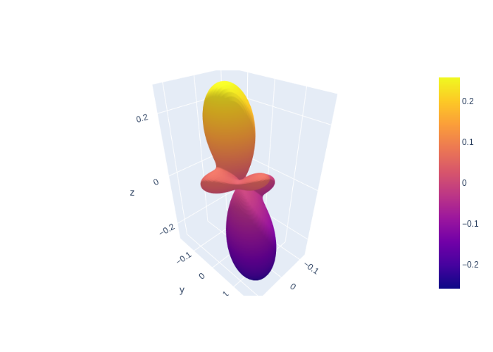
Plotting the Angular Shape
We can plot the angular “shape” of the states \(W(\theta, \phi)\) as they evolve over time Murray 2008:
, where \(Y_{J, m_J}(\theta, \phi)\) are the spherical harmonics for the state with total angular momentum \(J\) and projection \(m_J\).
Note: this only works for a single angular momentum state so will not produce the correct results for multiple \(F\)-states but will be correct for a single \(J\)-state.
In LASED we can plot the initial shape of the atomic state using the angularShape_0() function which takes the argument of theta and phi lists for the azimuthal (0 to 2\(\pi\)) and polar coordinates (0 to \(\pi\)) respectively as well as a state argument which equals either “g” or “e” depending on whether the angular shape of the excited or lower state in the LaserAtomSystem() will be calculated. The “angular shape” is the radius of the electron charge cloud as the
azimuthal and polar coordinate are varied.
[14]:
phi = np.linspace(0, np.pi, 100)
theta = np.linspace(0, 2*np.pi, 100)
W = helium_system.angularShape_0("g", theta, phi)
The angular shape can now be plotted using the plotting package desired. Here, I use Plotly. Before plotting, a mesh grid must be made for theta and phi and these must be converted to cartesian coordinates along with the radial coordinate calculated. A helpful function is the SphericalToCartesian function which is provided by LASED which takes the meshgrid and radius as inputs and provides x,y,z coordinates to be plotted.
[16]:
phi, theta = np.meshgrid(phi, theta)  # Create a mesh grid using numpy
x, y, z = las.SphericalToCartesian(W, theta, phi)  # Create cartesian coords
fig = go.Figure(data=[go.Surface(x=x, y=y, z=z)])  # Plot the result
fig.write_image("SavedPlots/tutorial3-HeAngularShapeDStatet=0.png")
Image("SavedPlots/tutorial3-HeAngularShapeDStatet=0.png")
[16]:
We can make a video for the evolution of the 3D-state’s electron cloud as it evolves over time in the laser-atom system. To do this, we have to generate the angular shape of the time evolution using the function angularShape_t which gives an array of angular shapes. Each angular shape must then be plotted and the images saved. Once all the images are saved they must be stitched together to create a video file. This can be done using any software package, ffmpeg is used here.
[20]:
phi = np.linspace(0, np.pi, 100)
theta = np.linspace(0, 2*np.pi, 100)
W_t = helium_system.angularShape_t("g", theta, phi)
phi, theta = np.meshgrid(phi, theta)
# Generate the images
for i, W in enumerate(W_t):
    x, y, z = las.SphericalToCartesian(W, theta, phi)
    # Plot the result
    fig = go.Figure(data=[go.Surface(x=x, y=y, z=z)])
    camera = dict(
    up=dict(x=0, y=0, z=1),
    center=dict(x=0, y=0, z=0),
    eye=dict(x=1.25, y=-1.25, z=1.5))
    fig.update_layout(scene_camera=camera)

    filenumber = "%0.5d"%i
    fig.write_image(f"Videos/3DShape" + filenumber + ".png", scale = 2.2)
[21]:
# Generate mp4 using ffpmeg
import subprocess

subprocess.call([
        'ffmpeg', '-framerate', '8', '-i', 'Videos/3DShape%05d.png', '-r', '30', '-pix_fmt', 'yuv420p',
        'He3DState1500mWCollFrame30deg.mp4'
    ])
[21]:
0